Feeder Protection Relay Operating Principles and Setting Calculations
- A feeder protection relay monitors current, voltage and fault direction to detect short circuits, earth faults and abnormal operating conditions. When the configured conditions are satisfied, it issues a trip command or alarm. Correct settings help isolate the faulty feeder selectively, limit the extent of an outage and provide backup protection for downstream equipment.
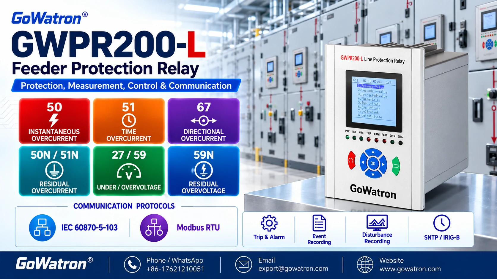
- This article uses the GoWatron GWPR200-L feeder protection relay to explain the main protection functions, operating principles and setting calculations. All numerical values are illustrative. Final settings must be based on the system fault study, instrument transformer data, protection coordination requirements and the manual for the installed relay version.
1. How Does a Feeder Protection Relay Work?
1.1 Current and Voltage Acquisition
- The GWPR200-L receives secondary signals from current transformers (CTs) and voltage transformers (VTs). It processes these signals to obtain phase currents, residual current, voltages and the phase relationships required by the protection elements.
Residual current is defined as:
\[ \underline I_{\mathrm{res}} = \underline I_A+\underline I_B+\underline I_C = 3\underline I_0 \]
- Here, \( I_0 \) is the zero-sequence current component, while \( I_{\mathrm{res}} \)is the residual current. Residual current may be measured using a core-balance current transformer (CBCT) or derived by summing three phase CT currents.
- A relay channel labelled “I0” does not necessarily indicate whether its settings represent \( I_0 \)or \( 3I_0 \). The input and setting definitions must be checked. The earth-fault example in this article uses\( I_{\mathrm{res}}=3I_0 \).
1.2 Fault Detection and Tripping
For a definite-time overcurrent element, the basic pickup condition is:
\[ I_{\mathrm{meas}}\geq I_{\mathrm{set}} \]
- Both quantities must use the same current reference. If this condition persists for the configured delay and all applicable permissive conditions are satisfied, the relay issues a trip command.
The total fault clearance time is:
\[ t_{\mathrm{clear}}=t_{\mathrm{relay}}+t_{\mathrm{CB}} \]
where:
- \( t_{\mathrm{relay}} \) is the time from fault inception to the relay trip output;
- \( t_{\mathrm{CB}} \) is the time from receipt of the trip command to interruption of the fault current.
The configured protection delay is therefore different from the total fault clearance time.
2. Main Feeder Protection Functions
2.1 Instantaneous Phase Overcurrent Protection (ANSI 50)
- The high-set instantaneous phase overcurrent element (ANSI 50) operates when current reaches its configured threshold, normally without an intentional time delay.
- Its setting must account for external faults assigned to downstream protection, transformer magnetising inrush, motor starting and other transient currents.
- This element may not cover the entire feeder. Time-delayed protection is therefore required to cover the remaining section.
2.2 Time Overcurrent Protection — Definite-Time Characteristic (ANSI 51)
- The definite-time element operates when current exceeds its pickup setting for a specified delay.
- The pickup setting must remain secure during maximum load conditions, while the delay must coordinate with downstream protection. This element can provide feeder protection and backup protection for downstream equipment.
2.3 Time Overcurrent Protection — Inverse-Time Characteristic (ANSI 51)
The inverse-time element operates faster as fault current increases. It is useful for coordinating feeder relays with downstream relays or fuses.
A commonly used IEC inverse-time equation is:
\[ t=TMS\times\frac{k}{(I/I_{\mathrm{set}})^\alpha-1} \]
where:
- \( t \) is the operating time in seconds;
- \( TMS \) is the time multiplier setting;
- \( I \) is the current applied to the element;
- \( I_{\mathrm{set}} \) is the pickup current;
- \( k \) and \( \alpha \)are curve constants.
The equation applies when\( I/I_{\mathrm{set}}>1 \). Both currents must be expressed on the same primary or secondary basis.
| Curve Type | \( k \) | \( \alpha \) |
| Standard inverse | 0.14 | 0.02 |
| Very inverse | 13.5 | 1 |
| Extremely inverse | 80 | 2 |
The available curves, time multiplier definition and minimum operating time must be checked against the manual for the installed GWPR200-L version.
2.4 Directional Overcurrent Protection (ANSI 67)
- Directional overcurrent protection evaluates both current magnitude and fault direction. Operation is permitted only when the overcurrent condition and the selected directional condition are satisfied.
- This function is useful in ring networks, dual-source systems and installations with distributed generation.
- The forward direction, polarising quantity, CT/VT polarity and relay characteristic angle (RCA) must be defined consistently. The RCA depends on the relay’s angle convention and polarising method and must not be copied between relay models without checking these definitions.
2.5 Residual Overcurrent Protection (ANSI 50N and 51N)
- ANSI 50N denotes the instantaneous residual overcurrent element; ANSI 51N denotes the time-delayed residual overcurrent element.
- These elements detect earth faults using residual current. The time-delayed element may use a definite-time or inverse-time characteristic, depending on the relay configuration.
- The pickup calculation must use the actual residual-current input ratio and the relay’s \( I_0 \) or\( 3I_0 \)definition.
2.6 Directional Earth-Fault Protection (ANSI 67N)
- Directional earth-fault protection combines an earth-fault current criterion with directional discrimination to improve selectivity.
- The RCA and polarising method depend on the neutral earthing arrangement. Settings for resistance-earthed, unearthed and resonant-earthed systems are not interchangeable.
2.7 Undervoltage, Overvoltage and Residual Overvoltage Protection (ANSI 27/59/59N)
| Protection Function | ANSI Designation | Purpose |
| Undervoltage protection | 27 | Detects sustained low-voltage conditions |
| Overvoltage protection | 59 | Detects sustained high-voltage conditions |
| Residual overvoltage protection | 59N | Detects elevated residual voltage, commonly associated with earth faults |
- Depending on the manufacturer and measurement arrangement, ANSI 59N is also referred to as neutral overvoltage or zero-sequence overvoltage protection. The measured quantity and any \( U_0 \) or \( 3U_0 \)scaling must be checked.
- Voltage thresholds, delays and alarm or trip assignments must suit the system requirements and VT connections.
2.8 Voltage-Supervised Overcurrent Protection — Undervoltage and Negative-Sequence Voltage Supervision
- Voltage supervision typically combines undervoltage and negative-sequence voltage criteria. A low-voltage condition or elevated negative-sequence voltage provides permission for the associated overcurrent element.
- The current, time-delay and any applicable directional conditions must also be satisfied before tripping.
- The measured voltage quantities, logic and response to VT circuit failure must be verified against the relevant GWPR200-L manual.
3. Feeder Protection Setting Methods
3.1 Converting Primary Current to Secondary Current
\[ I_{\mathrm{set,sec}} = \frac{I_{\mathrm{set,pri}}}{n_{\mathrm{CT}}} \]
\[ n_{\mathrm{CT}}=\frac{400}{5}=80 \]
\[ I_{\mathrm{set,sec}}=\frac{320}{80}=4.00\ \mathrm A \]
3.2 Low-Set Time Overcurrent Protection (ANSI 51) Pickup Calculation
- This preliminary calculation applies to the low-set stage of either a definite-time or an inverse-time element.
- The pickup setting must remain above the maximum expected load and allow the element to reset after a temporary overcurrent:
\[ I_{\mathrm{set,pri}} \geq \frac{K_{\mathrm{rel}}K_{\mathrm{load}}}{K_{\mathrm{reset}}} I_{\mathrm{load,max,pri}} \]
- \( K_{\mathrm{rel}} \) is the security factor, providing a setting margin;
- \( K_{\mathrm{load}} \)allows for additional load growth, motor starting or load restoration, including cold-load pickup where applicable;
- \( K_{\mathrm{reset}} \) is the reset ratio, defined as reset current divided by pickup current;
- \( I_{\mathrm{load,max,pri}} \)is the maximum primary load current.
3.3 Overcurrent Protection Sensitivity Check
\[ K_{\mathrm{sen}} = \frac{I_{\mathrm{fault,min,pri}}}{I_{\mathrm{set,pri}}} \]
- \( I_{\mathrm{fault,min,pri}} \) must be the minimum current flowing through the same protection element for the relevant fault type and system configuration.
- The same primary or secondary basis must be used for both currents. The equation above uses primary values.
- The required sensitivity factor depends on the protection duty, earthing arrangement and applicable design requirements. It should be specified by the project.
3.4 High-Set Instantaneous Overcurrent Protection (ANSI 50) Setting Calculation
\[ I_{\mathrm{high,pri}} \geq K_{\mathrm{rel}}I_{\mathrm{external,max,pri}} \]
- Here, \( I_{\mathrm{external,max,pri}} \)is the maximum primary current flowing through the relay for the relevant external fault.
- The setting must then be checked against internal fault coverage, transient currents, and CT accuracy, saturation and transient performance.
3.5 Time Overcurrent Protection (ANSI 51) Coordination — Definite-Time and Inverse-Time
\[ t_{\mathrm{up}} \geq t_{\mathrm{down}}+CTI \]
- where \(CTI\) is the coordination time interval. It must allow for downstream circuit-breaker clearance time, relay timing tolerances and an appropriate margin.
- For inverse-time protection, the coordination time interval must be checked across the relevant fault-current range rather than at a single current value.
4. GWPR200-L Setting Examples
4.1 Phase Overcurrent Protection (ANSI 50/51)
- Consider an 11 kV feeder with 400/5 A CTs, a maximum primary load current of 240 A and a minimum remote-end primary phase-fault current of 1,800 A under the least favourable system configuration.
| Setting Item | Illustrative Calculation | Result |
| Low-set primary pickup | \( 1.2\times240/0.9 \) | 320 A |
| Low-set secondary pickup | \( 320/80 \) | 4.00 A |
| Low-set sensitivity factor | \( 1800/320 \) | 5.63 |
| Definite-time delay | 0.30 s downstream time + 0.30 s CTI | 0.60 s |
| High-set primary pickup | 3,000 A maximum external fault current × 1.3 | 3,900 A |
| High-set secondary pickup | \(3900/80\) | 48.75 A |
- The low-set calculation uses \( K_{\mathrm{rel}}=1.2 \), \( K_{\mathrm{reset}}=0.9 \) and \( K_{\mathrm{load}}=1.0 \). The high-set calculation uses \\( K_{\mathrm{rel}}=1.3 \).
- The sensitivity factor is calculated by dividing the minimum remote-end primary phase-fault current of 1,800 A by the low-set primary pickup of 320 A.
If the minimum primary current for a selected internal fault is 6,000 A, its ratio to the high-set pickup is:
\[ 6000/3900=1.54 \]
- An internal fault nearer the source may produce more current than a more distant external fault because of the lower equivalent fault-path impedance.
- High-set coverage must be established by calculating fault currents at different feeder locations. The current ratio cannot be converted directly into a percentage of feeder length.
- All candidate settings must be checked against the relay’s setting range and resolution, as well as CT accuracy, saturation and transient performance.
4.2 Time Overcurrent Protection — Inverse-Time Coordination (ANSI 51)
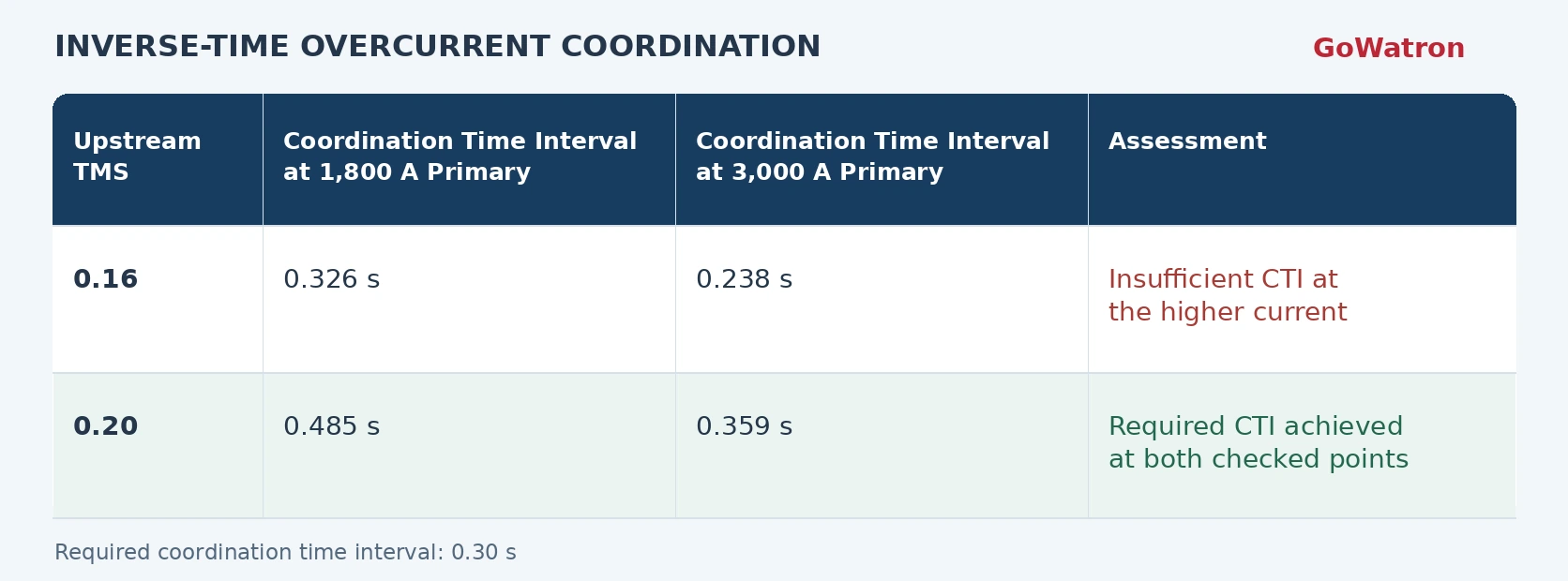
This example assumes that the same primary fault current flows through both relays and that no other element operates first.
Final coordination requires assessment of the full relevant current range, curve tolerances and equipment thermal withstand capability.
4.3 Residual Overcurrent Protection (ANSI 50N and 51N)
- Assume a resistance-earthed system with a 100/1 A CBCT, a maximum normal primary residual current of 8 A and a minimum primary earth-fault residual current of 100 A.
- A security factor\( K_{\mathrm{rel}}=1.5 \) applied to the 8 A maximum normal primary residual current gives a preliminary minimum primary pickup of 12 A. Selecting a primary pickup of 20 A gives:
\[ I_{\mathrm{res,set,sec}}=\frac{20}{100}=0.20\ \mathrm A \]
\[ K_{\mathrm{sen}}=\frac{100}{20}=5 \]
- The delay must coordinate with adjacent earth-fault protection. External-fault spill current and transient effects must also be checked.
- This example uses \( I_{\mathrm{res}}=3I_0 \) and must not be applied directly to unearthed or resonant-earthed systems.
4.4 Directional Overcurrent and Directional Earth-Fault Protection (ANSI 67/67N)
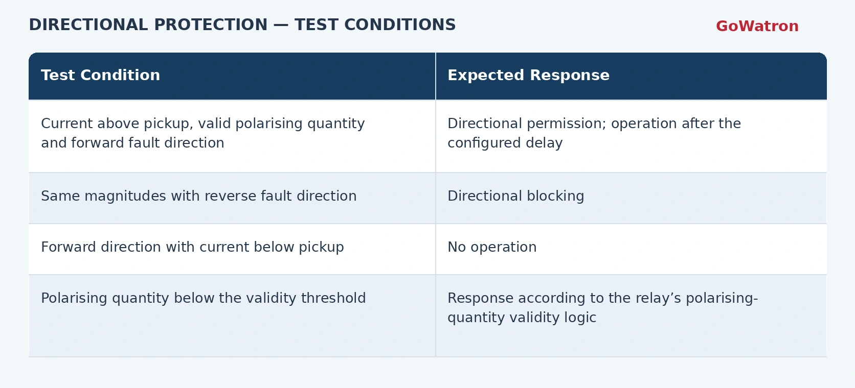
- For example, if calculated forward-fault angles cluster around \( 45^\circ \) under the specified convention, this can guide RCA selection and boundary testing. It is not a universal GWPR200-L setting.
- Directional earth-fault tests must additionally account for the neutral earthing arrangement and the polarity and scaling of the residual voltage used for polarisation, including whether it represents \( U_0 \), \( 3U_0 \) or an inverted quantity.
4.5 Voltage-Supervised Overcurrent Protection
All voltages in this example are secondary quantities.
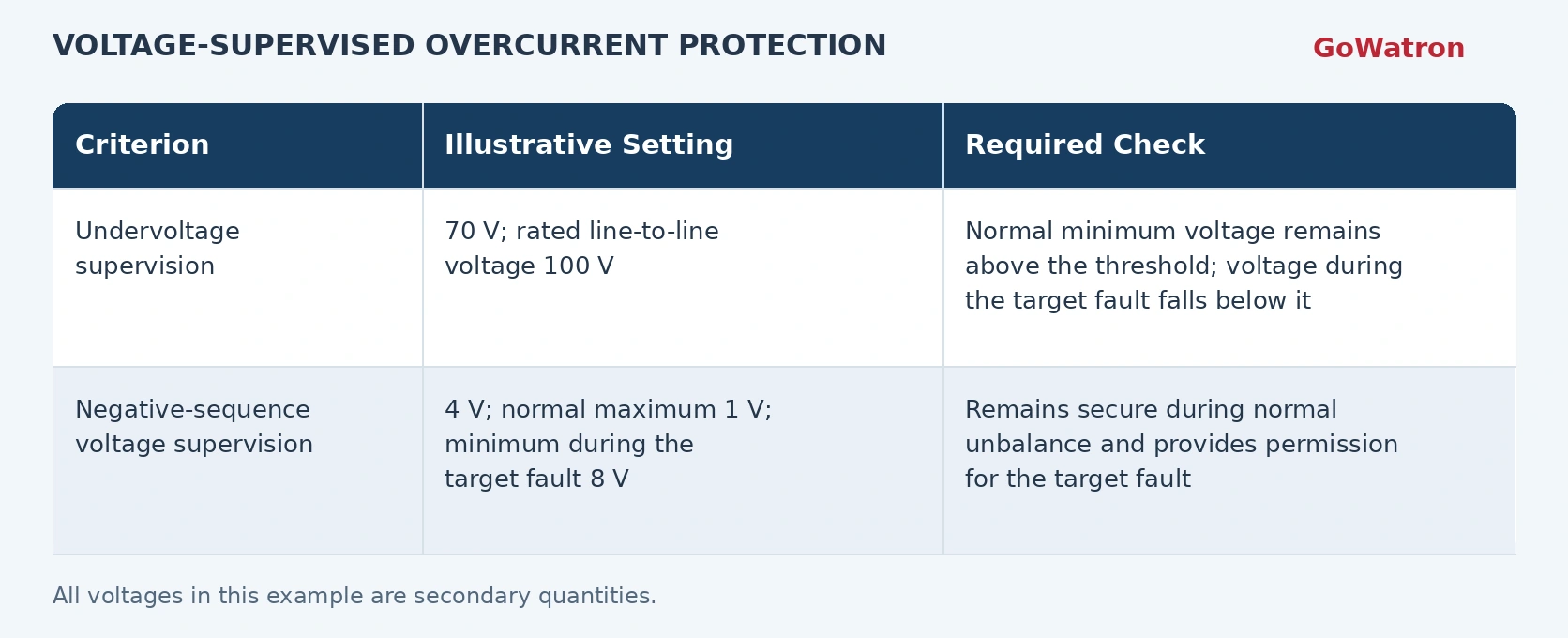
- The negative-sequence values must all use the same voltage definition and reference base. Phase-voltage and line-to-line-voltage values must not be used interchangeably.
- These values demonstrate the selection method. Actual thresholds must be derived from normal and fault voltage studies, with the response to VT circuit failure verified separately.
5. Setting and Commissioning Checks
Before placing the GWPR200-L feeder protection relay into service:
- Confirm CT/VT ratios, rated inputs and primary or secondary setting conventions.
- Check security during maximum load, motor starting and load restoration, including cold-load pickup where applicable.
- Verify sensitivity under minimum fault-current conditions.
- Check upstream and downstream coordination and equipment thermal withstand capability.
- Confirm directional conventions, polarising-quantity validity logic, voltage supervision and the response to VT circuit failure.
- Use secondary injection and trip-circuit tests to verify pickup, reset, operating time and the complete tripping path.


